2014년, 이안 굿펠로우(Ian Goodfellow)에 의해 고안된 GAN(Generative Adversarial Network)은 생성 모델과 딥러닝 분야에 큰 혁신을 불러일으켰습니다. 특히, GAN은 이미지 생성, 스타일 변환, 영상/음성 합성 등 다양한 분야에서 우수한 성능을 보였으며, 최근 이상탐지 분야에서도 사용되고 있습니다. 이번 글에서는 이상탐지에서의 GAN의 활용에 대해 다루어 보겠습니다.
생성 모델과 판별 모델
기계 학습에서 분류(Classification) 문제를 해결하기 위한 알고리즘은 생성 모델(Generative Model)과 판별 모델(Discriminative Model) 크게 2가지 종류가 있습니다. 판별 모델은 분류 경계를 찾는 것을 목적으로 학습하는 반면에, 생성 모델은 데이터의 분포를 학습합니다. 예를 들어, 판별 모델 관점에서 개와 고양이 분류는 개와 고양이의 샘플 데이터로부터 각각의 특징을 학습한 후, 두 클래스(개, 고양이)의 특징을 구분 짓는 경계선을 찾는 방식으로 진행됩니다. 반면에, 생성 모델을 활용한 분류는 개와 고양이의 샘플 데이터가 따르는 분포를 학습하여 두 집단을 구분하고, 학습이 끝난 후 모델을 활용하여 유사한 데이터를 생성합니다.
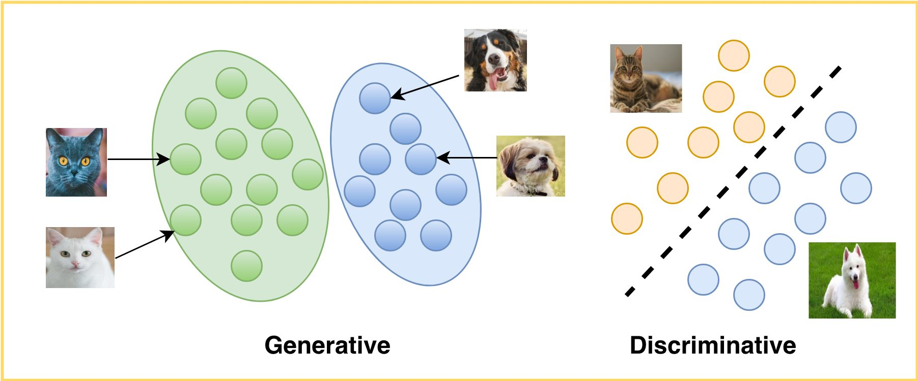
<생성 모델과 판별 모델 비교>
GAN 개념
GAN(Generative Adversarial Network)은 ‘진짜 같은 가짜 데이터’를 생성하는 대표적인 생성 모델입니다. GAN이라는 이름에서 알 수 있듯이, GAN은 두 개의 모델이 적대적(Adversarial)으로 경쟁하듯이 학습하면서, 진짜 같은 가짜 데이터를 생성하는(Generative) 신경망 모델(Network) 입니다. 여기서 ‘생성’은 실제 데이터 분포에 근사하도록 학습하는 것을 전제로 합니다. 즉, 실제 데이터 분포에 근사하게 모델을 학습하면, 유사한 샘플 데이터를 생성할 수 있습니다. 그리고, ‘적대적(Adversarial)’은 GAN 모델의 학습 원리를 상징하는 용어이며, 생성자(Generator)와 구분자(Discriminator) 두 개의 모델을 경쟁하여 성능을 향상시키는 방향으로 학습하는 것을 의미합니다.
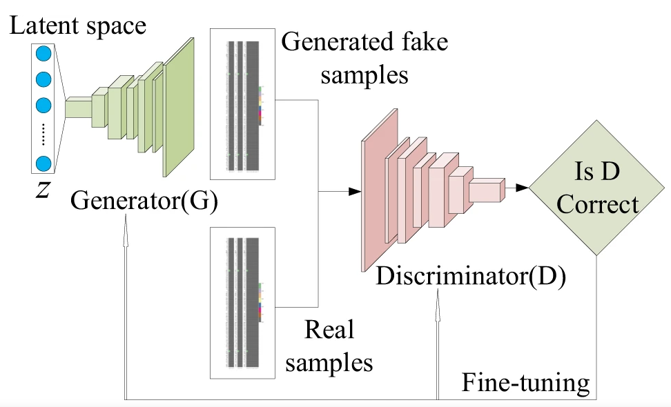
<GAN 아키텍처>
GAN 기반 이상탐지
이상탐지(Anomaly Detection)는 데이터에서 비정상적인 값을 탐지하는 것을 의미합니다. 이상탐지를 위한 기법은 분포, boxplot 등을 활용하여 이상치를 찾는 통계적 방법부터 모델을 이용하여 예측하는 방법까지 다양합니다. 최근에는 이미지 데이터 상의 이상부분을 탐지하기 위하여 GAN을 이용한 연구가 진행되고 있습니다. AnoGAN, GANomaly 등 이상탐지를 위한 다양한 GAN 기반 모델들이 연구되었으며, 여기서는 GANomaly를 소개하도록 하겠습니다.
GANomaly는 생성자(Generator)가 Encoder-Decoder-Encoder의 구조를 갖습니다. 구성된 네트워크 수가 많은 만큼 Generator의 손실 함수(Loss Function)도 여러 개 Loss (Encoder Loss, Contextual Loss, Adversarial Loss)의 합으로 구성됩니다.
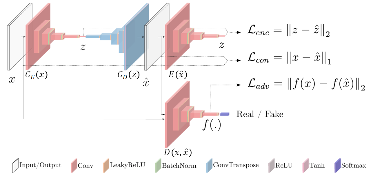
<GANomaly 아키텍처>
아래는 GANomaly의 Generator Loss를 구현한 코드입니다. 코드는 MNIST의 ‘1’과 ‘7’을 각각 정상/비정상으로 간주하고 분류한 알고리즘을 구현한 것입니다. Encoder Loss는 G_E(x)의 출력값과 E(x_hat)의 출력값에 대한 MSE로 정의됩니다. Contextual Loss는 G_E(x)의 출력값과 E(x_hat)의 출력값에 대한 MAE로 정의됩니다. Adversarial Loss는 D(x, x_hat)의 출력값에 대한 MSE로 계산됩니다.
이 3개의 Loss에 가중치를 각각 곱해서 합한 값을 최종적으로 Generator Loss로 사용합니다.
class EncLoss(keras.layers.Layer):
	def __init__(self, **kwargs):
		super(EncLoss, self).__init__(**kwargs)

	def call(self, x, mask=None):
		ori = x[0]
		gan = x[1]
		return K.mean(K.square(g_e(ori) - encoder(gan)))

	def get_output_shape_for(self, input_shape):
		return (input_shape[0][0], 1)

class CntLoss(keras.layers.Layer):
	def __init__(self, **kwargs):
		super(CntLoss, self).__init__(**kwargs)

	def call(self, x, mask=None):
		ori = x[0]
		gan = x[1]
		return K.mean(K.abs(ori - gan))

	def get_output_shape_for(self, input_shape):
		return (input_shape[0][0], 1)

class AdvLoss(keras.layers.Layer):
	def __init__(self, **kwargs):
		super(AdvLoss, self).__init__(**kwargs)

	def call(self, x, mask=None):
		ori_feature = feature_extractor(x[0])
		gan_feature = feature_extractor(x[1])
		return K.mean(K.square(ori_feature - K.mean(gan_feature, axis=0)))

	def get_output_shape_for(self, input_shape):
		return (input_shape[0][0], 1)

input_layer = layers.Input(name='input', shape=(height, width, channels))
gan = g(input_layer) # g(x)
adv_loss = AdvLoss(name='adv_loss')([input_layer, gan])
cnt_loss = CntLoss(name='cnt_loss')([input_layer, gan])
enc_loss = EncLoss(name='enc_loss')([input_layer, gan])

gan_trainer = keras.models.Model(input_layer, [adv_loss, cnt_loss, enc_loss])

# loss function
def loss(yt, yp):
	return yp

losses = {
	'adv_loss': loss,
	'cnt_loss': loss,
	'enc_loss': loss,
}

lossWeights = {'cnt_loss': 20.0, 'adv_loss': 1.0, 'enc_loss': 1.0}

# compile
gan_trainer.compile(optimizer = 'adam', loss=losses, loss_weights=lossWeights)
Loss 정의 후, ‘d’(=Discriminator)를 학습가능하게 설정하고 ‘train_on_batch’ 메소드를 사용하여 학습합니다. 그리고 구분자 ‘d’를 학습 범위에서 제외하고, 생성자 ‘gan_trainer’를 학습시킵니다. 이 과정을 iteration 수만큼 반복합니다.
for iin range(niter):
	### get batch x, y ###
	x, y = train_data_generator.__next__()

	### train disciminator ###
	d.trainable =True

	fake_x = g.predict(x)

	d_x = np.concatenate([x, fake_x], axis=0)
	d_y = np.concatenate([np.zeros(len(x)), np.ones(len(fake_x))], axis=0)

	d_loss = d.train_on_batch(d_x, d_y)

	### train generator ###
	d.trainable =False
	g_loss = gan_trainer.train_on_batch(x, y)

	if i % 50 == 0:
		print(f'niter:{i+1}, g_loss:{g_loss}, d_loss:{d_loss}')
학습이 끝난 후, 테스트 데이터를 입력하여 각 네트워크 별 예측값을 구하고, 이 예측값들을 이용하여 이상탐지 점수(Anomaly Score)를 구합니다. 이상탐지 점수는 논문에 따라 Encoder Loss에 기반하여 G_E(x)의 예측값과 E(G(x))의 예측값에 대한 SSE로 정의합니다. 그리고, Min-max 정규화를 통해 0부터 1사이 범위로 변환합니다.
encoded = g_e.predict(x_test)
gan_x = g.predict(x_test)
encoded_gan = g_e.predict(gan_x)
score = np.sum(np.square(encoded - encoded_gan), axis=-1)
score = (score - np.min(score)) / (np.max(score) - np.min(score))# map to 0~1
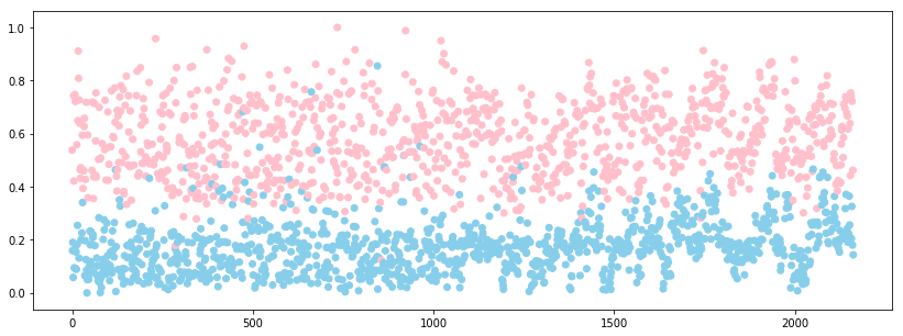
최종적으로 Min-max 정규화된 이상탐지 점수(Anomaly Score)를 산점도로 시각화하면 아래 그림과 같습니다. 이상탐지 점수가 약 0.3일 때를 기준으로 두 클래스가 구분되는 것을 볼 수 있습니다. 따라서, 약 0.3 정도를 임계값으로 정하여서 테스트 데이터에 대한 이상 여부를 판단할 수 있습니다.
import matplotlib.pyplot as plt
from pylab import rcParams
rcParams['figure.figsize'] = 14, 5
plt.scatter(range(len(x_test)), score, c=['skyblue' if x == 1 else 'pink' for x in y_test])
결 론
이번 글에서는 이상탐지를 위한 GAN 모델을 설명하기에 앞서, 생성 모델과 판별 모델의 차이와 GAN 개념을 설명하였습니다. 그리고 다양한 이상탐지를 위한 GAN 모델 중, GANomaly 모델을 소개하였습니다. 특히, GANomaly의 전체적인 아키텍처와 손실 함수 정의, 테스트 및 시각화를 중점적으로 다루었습니다.
다음 글에서는 CNN기반 이상데이터 분류에 대해 다루어 보도록 하겠습니다.
Reference
https://ratsgo.github.io/generative%20model/2017/12/17/compare/
https://learnopencv.com/generative-and-discriminative-models/
https://dreamgonfly.github.io/2018/03/17/gan-explained.html
Dan, Y., Zhao, Y., Li, X., Li, S., Hu, M., & Hu, J. (2020). Generative adversarial networks (GAN) based efficient sampling of chemical composition space for inverse design of inorganic materials. npj Computational Materials, 6, 1-7.
Akçay, S., Atapour-Abarghouei, A., & Breckon, T. (2018). GANomaly: Semi-Supervised Anomaly Detection via Adversarial Training. ACCV.
https://github.com/leafinity/keras_ganomaly